vscsiStats into the third dimension: Surface charts!
How could I ever have missed it… vscsiStats. A great tool within vSphere which enables you to see VM disk statistics. And not only latency and number of IOPs… But actually very cool stuff like blocksizes, seekdistances and so on! This information in not to be found in esxtop or vCenter performance graphs… So we have to rely on once more on the console…
UPDATE: Available now: vscsiStats in 3D part 2: VMs fighting over IOPS !
UPDATE2: Build your own 3D graphs! Check out vscsiStats 3D surface graph part 3: Build your own!
I will not be going into the details of setting up how to use vscsistats. There are plenty of blogposts on that, for example this great post on Gabes Virtual World
vscisStats is a REALLY cool tool. Though exciting as vscsistats may be, it is and remains a tool which measures over time and then outputs a number of histograms of a certain virtual disk. All are basically mean values over time.
Those who have read my performance report on the Sun 7000 storage (see Breaking VMware Views sound barrier with Sun Open Storage) will know I am a big fan of surface charts. Basically vscsiStats is a perfect tool for integration into 3D graphs.
The idea is that vscsistats should be used to create the histograms over let’s say 30 seconds. Then shoot another 30 seconds, then another… After 20 “samples” we put all histograms into a surface area chart and voila! We have disk statistics visible as time passes by.
TO THE LAB!
It is once again testing time! After getting the first results out of vscsiStats, I wrote a very basic piece of script to get several measurements right behind each other. Just call it using three parameters (WorldGroupID, HandleID, sampletime):
echo Recreating the output file

rm -f out1.csv

touch out1.csv
echo Running stats
/usr/lib/vmware/bin/vscsiStats -w $1 -i $2 -s
for i in $(seq 1 1 21)
do
sleep $3
/usr/lib/vmware/bin/vscsiStats -w $1 -i $2 -p all -c >>out1.csv
/usr/lib/vmware/bin/vscsiStats -w $1 -i $2 -r
done
/usr/lib/vmware/bin/vscsiStats -w $1 -i $2 -x
EDIT: Thanks to NiTRo (from www.hypervisor.fr ) for the edit in the “for” command to get it ESXi compatible!
Basically this script starts measurements on a single virtual disk, after 30 seconds the data is added to a file in the csv format and the statistics get a reset. This process is repeated 21 times. So I end up with 21 sets of histograms, each 30 seconds apart.
Now the magic Excel comes in. Drawing the histograms right after each other makes them interconnect-able using a surface chart.
ENOUGH TALK… ON TO THE OUTPUT!
Once the Excel is built, you can quickly import different vscsiStats outputs into the Excel form, and the 3D graphs will immediately show you the measured values in 3D! I have used standard colors for different graphs: blue for I/O, green for READS and red for WRITES. Check it out:
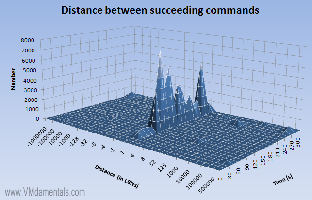
As you can see, through time there is a very clear “edge” along the +1 line. This indicates linear I/O. Cool right! On to more examples…
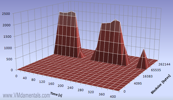
EXAMPLE 1: vCenter Bootdisk
This is what a vCenter server bootdisk is doing all day:
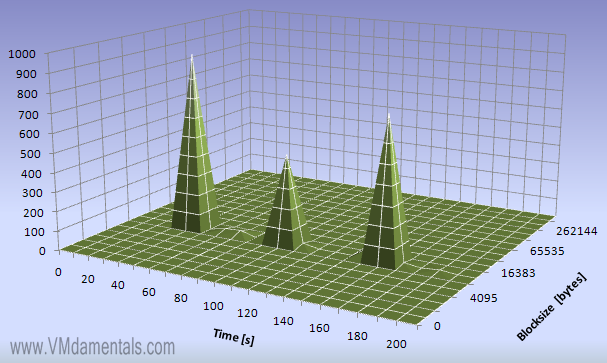
Basically the disk is idle for reads, but every 60 seconds there is a read burst of 8192 byte blocks, between 500 and 900 reads are performed.
Writes are significantly less, but more regular. Most writes appear to be 4096 byte blocks, some smaller.
So how about randomness of these reads/writes? Well, check this out:
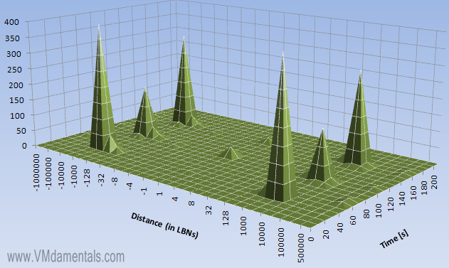
… You can clearly see the three recorded bursts laying in the graph. These reads are pretty much random, since almost all have a distance of around 1000 logical blocks.
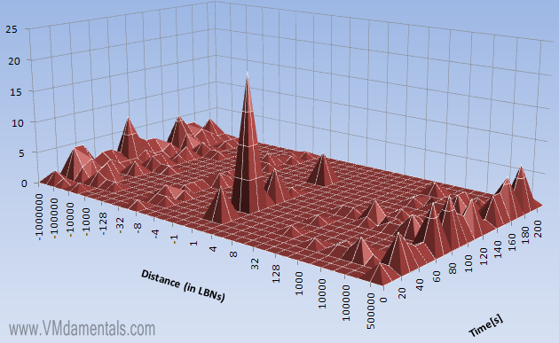
Writes are more of a mishmash. Most writes are fully random (the edges around +500.000 and -500.000), but some of the writes are linear (the peaks in the center of the graph). Especially the peak in the center of the graph at 60 seconds. Now check out the previous writes graph at 60 seconds: There is a peak visible there also, at a very small blocksize of only 1024 byte blocks. My guess would be the system (for some reason) decided to write many small blocks sequentially to disk. This definitely shows the power of vscsiStats in 3D: in a single large data fetch and a single histogram this behavior would have been missed!
EXAMPLE 2: Streaming a DVD from a fileserver
Let’s see what happens on a virtual disk which is streaming a DVD:
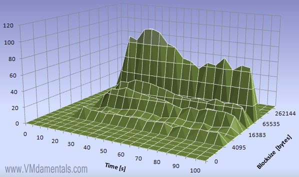
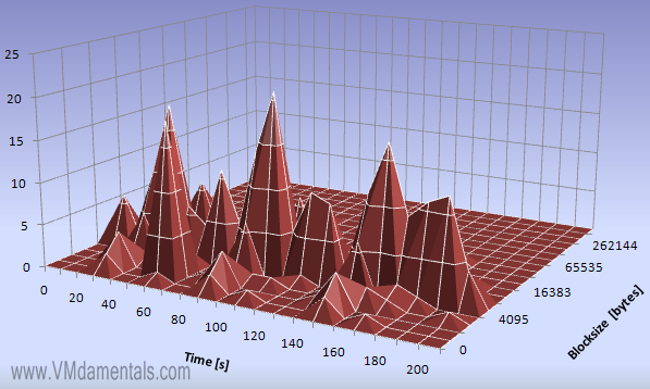
When streaming data from a file server you can see several block sizes are used. Peaks are visible at 4096, 16384 and 65536, exactly 4K, 16K and most at 64K blocks. It appears the blocks are neatly sized as-needed. I’d expect the reads to be sequential, but how sequential are they really?

Hmm. The distance graph shows that there is a massive linear component (edge in the center of the graph at +1). But there are also two edges visible, one at -128 and one at +128 logical blocks.
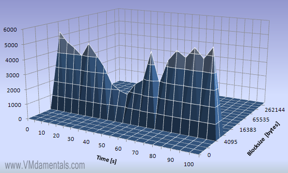
EXAMPLE 3: Large file reading and writing
Another example is heavy file writing and reading. In this example, I use my file server to copy a large file back and forth a few times between two virtual disks using a batch file:
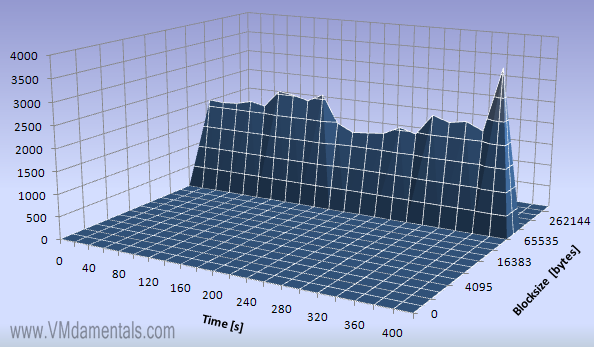
The file server is busy busy busy… I see a constant I/O activity at 64K blocks…
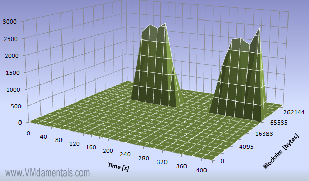
Here you can see the reads… It now becomes clear the server reads, then appears to wait, then reads again.
Looking at the writes we see the same behavior, but exactly when the reading is idle. Bingo, my batch file does writes-then-reads-then-writes-then-reads-then-writes…

Not much exciting to see in the read distance… reads are 100% sequential.

Writes are a 100% sequential as well…

Read latency is at a very stable 5 [ms]…

Uhm! Write latency is around 50 [ms]. It is apparent my storage device is not the fastest around (anyone got an unused EMC AX4-5 somewhere? 😉 )
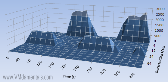
Now this one is funny… Because the write latency is much higher, so are the number of outstanding I/Os for writes… In the combined I/O graph (blue!) it is clearly visible.
EXAMPLE 4: Generating a random read/write using IOmeter
Just because I can… I decided to run an IOmeter load on 4K blocks, 50% reads 50% writes, 100% random. This is what I got:

Interestingly, IOmeter is not showing a sustained I/O bandwidth, probably because I choose to have no outstanding I/Os in this test. All performed I/Os are neatly at 4096 byte blocks though, as specified within IOmeter.

The read distance is exactly what was to be expected: at 50% sequential and 50% random, the edges in the center and in the corners are clearly visible.

For writes, the same story as for the reads: at 50% sequential and 50% random this is expected behavior.

Write Latency is low. This is probably because the number of outstanding I/Os was set to zero, effectively not performing writes if another write is pending. As a result, latency in writes is low in this test.

Reads are more of a mixed bag: Some reads appear to finish quicker than other, it is either 0,5 [ms] or 10[ms]. This is probably due to the fact that 50% of the reads are performed sequential, 50% is random (slower). Cool!
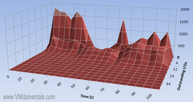
EXAMPLE 4b: Example 4, but with 12 outstanding I/O’s
I just HAD to run one other test! It is basically the same test as above, but now I tell IOmeter to use up to 12 outstanding I/O’s:
Now that we allow some I/O to be outstanding, you can clearly see much more data is moved, and also in a more regular fashion when compared to example 4.

Looking at the outstanding reads, we see that the virtual disk actually is crammed with reads: At almost all times it has 12 reads outstanding (IOmeter just keeps filling the buffer)
In writes, we see less outstanding I/O’s. Really up to 12 outstanding, but most of the time there are less outstanding I/O than the maximum configured.
CONCLUSION
The vscsiStats command is a really really great tool to examine disk-workloads on virtual servers. From there on you could potentially optimize your stripe/segment sizes on storage arrays, for example when you are tuning RAID5 sets for optimizing writes (also see Throughput part2: RAID types and segment sizes“).
But adding the third dimension gives an insight about varying behavior through time. Not always needed (like some VMs which perform very steady through time), but especially when workloads vary on a virtual disk it might be worthwhile to look at things with a little more depth!


 LinkedIn
 Twitter
[…] This post was mentioned on Twitter by Eric Sloof and Sven Huisman, VMware Architect. VMware Architect said: #VMware #News vscsiStats into the third dimension: Surface charts!: Those who have read my performance report on t… http://bit.ly/bC4mWh […]
Great article. Looks like vscsiStats can provide a wealth of info. Is there a particular version required for this? When I ran the script, I get mostly 0’s. In the first column I will occasionally get a number to the 14th power and the second column is all 0’s.
adam
I think vscsiStats was available already in ESX 3.5 (not sure though). If you run vscsiStats to monitor an (almost) idle disk, you’ll end up getting almost all zeros. Nice test is to look at a VM’s bootdisk using vscsiStats, then reboot the VM. You’ll see the boot proces as time passes by…
THose are killer graphs. Can you explain in more detail how to get the CSV data into a format Excel can use to plot, and what graph settings you used to produce those beautiful plots?
I am planning to release a third blogpost on the vscsiStats subject. I am thinking to include some simple form of the Excel file I use… In that file you can simply import files you “shoot” with the script and the graphs show instantaneously… 🙂
Sweet!!! Can I run your scripts on a vMA?
Hi Derek. As far as I know the vMA has no support for vscsiStats. I’m not even sure ESXi supports it (haven’t tested).
[…] is going to be way cool this year! Eric Sloof will be using some of my 3D graphs (see ‘vscsiStats into the third dimension: Surface charts!‘ and ‘vscsiStats in 3D part 2: VMs fighting over IOPS‘). I cannot wait to hear […]
[…] vscsiStats data using 3D surface charts is awesome. I love […]
Fun with vSCSIStats output: http://bit.ly/aLbpwE
RT @joshuatownsend Fun with vSCSIStats output: http://bit.ly/aLbpwE
I like these charts a lot. Nice work!
I will have to see if I can get my PowerCLI script modified to draw surface charts now 🙂
Hi Michael,
I am planning to release a basic version of my Excel file soon. That file simply “eats” output of the vscisStats command and insantaneously outputs the surface charts 🙂
[…] from the vcsiStats tool. I use a simple Excel sheet for this. Using the script I described in vscsiStats into the third dimension: Surface charts! , you can import the files outputted into excel and see the Excel chart […]
So the shell script is acting weird on it..it just goes through one loop then exits. I cut and paste exactly from your blog.
Hi,
The script shoudl work… It is a simple for loop which repeats the measurements 20 times… Maybe some windows ^M chars were accidentally sneaked in somewhere?
This post rocks!
[…] Eric has one of my fun 3D vscisiStats stuff included in his presentation! See http://www.vmdamentals.com/?p=722 or vscsiStats 3D surface graph part 3: Build your own! to build your own like these: On the […]
[…] vscsiStats into the third dimension: Surface charts! […]
FYI i had to replace “for i in {1..21}” by “for i in $(seq 1 1 21)” to make it works on esxi
Anyway, it totally rocks 🙂
Thank you NiTRo. Great this works on ESXi as well! That’s the problem of my homelab… Time to convert one of my ESX nodes to ESXi I guess 🙂
Yes it’s time consuming but upgrades and maintenance is so easy with ESXi that it really worth it 🙂
[…] post on using Microsoft Chart Controls to visualise vscsiStats data and Eric Zandboer even has cool 3d Excel charts! Categories: VCAP, VMware, Virtualisation Tags: esxtop, resxtop, vscsiStats Comments (0) […]
[…] has no means of measuring block sizes, you could use vscsiStats (for examples you could look at vscsiStats into the third dimension: Surface charts!). Use this tool to find out if you actually have VMs performing “large” I/O’s. In […]
[…] If the workload appears to be very high for this virtual machine, you may look into a command line tool called vscsiStats. This tool can give great insight in reads and writes, block sizes and latencies your VM encounters/generates. See VMdamentals.com: vscsiStats into the third dimension. […]
[…] vscsiStats into the third dimension: Surface charts! […]
[…] Learn how to understand vscsiStats output and format them into an easy to understand language @ vmdamentals.com […]